110 / 85#> [1] 1.294118Pidä oma muistikirjasi auki Positronissa. Demokoodi etenee luennon järjestyksessä. Harjoittele omassa tiedostossasi ja avaa mallikoodi vasta oman kokeilun jälkeen.
Laske sokki-indeksi konsolissa. Tallenna seuraavaksi arvot nimillä ja käytä niitä laskussa.
110 / 85#> [1] 1.294118syke <- 110
systolinen <- 85
syke / systolinen#> [1] 1.294118sykkeet <- c(72, 88, 110, 95)
mean(sykkeet)#> [1] 91.25Avaa ohje Positronin Help-paneeliin.
?meanTallenna sykearvo 110 ja systolinen paine 85 koodisoluun. Laske sokki-indeksi, kirjoita tuloksesta muistiinpano solun alle ja avaa Preview.
syke <- 110
systolinen <- 85
syke / systolinenAja oman muistikirjasi valmistelusolu ennen esimerkkejä. Se lataa tidyverse-paketit ja luo muuttujan news NHSRdatasets-paketin synteettisestä aineistosta.
# Synteettisen opetusaineiston valmistelu. Muokkaukset opetetaan päivänä 2.
library(tidyverse)

news <- NHSRdatasets::synthetic_news_data |>
  mutate(
    sex = factor(male, levels = 0:1,
                 labels = c("Female", "Male")),
    oxygen = factor(sup, levels = 0:1,
                    labels = c("Room air", "Oxygen")),
    avpu = factor(alert, levels = 0:3,
                  labels = c("A", "V", "P", "U")),
    outcome = factor(died, levels = 0:1,
                     labels = c("Survived", "Died")),
    risk = cut(NEWS, breaks = c(-Inf, 4, 6, Inf),
               labels = c("Low (0-4)", "Medium (5-6)",
                          "High (7+)"))
  ) |>
  select(age, sex, NEWS, risk, resp, sat, oxygen,
         syst, dias, pulse, temp, avpu, died, outcome)
Tutki rivejä, sarakkeiden tyyppejä, tunnuslukuja ja ryhmäkokoja.
news#> # A tibble: 1,000 × 14
#> age sex NEWS risk resp sat oxygen syst dias pulse temp avpu
#> <int> <fct> <int> <fct> <int> <int> <fct> <int> <int> <int> <dbl> <fct>
#> 1 68 Female 3 Low (0… 26 96 Room … 150 98 78 36.8 A
#> 2 94 Male 1 Low (0… 18 96 Room … 145 67 62 35 A
#> 3 85 Female 0 Low (0… 18 96 Room … 169 69 54 36.2 A
#> 4 44 Male 0 Low (0… 17 96 Room … 154 106 80 36.9 A
#> 5 77 Female 1 Low (0… 20 95 Room … 122 67 62 36.4 A
#> 6 58 Female 1 Low (0… 20 98 Room … 146 106 73 35.3 A
#> 7 25 Female 4 Low (0… 12 99 Room … 65 42 72 35.6 A
#> 8 69 Female 0 Low (0… 16 97 Room … 116 56 90 37.2 A
#> 9 91 Female 1 Low (0… 16 99 Room … 162 72 60 35.5 A
#> 10 70 Female 1 Low (0… 16 97 Room … 132 96 67 35.3 A
#> # ℹ 990 more rows
#> # ℹ 2 more variables: died <int>, outcome <fct>glimpse(news)#> Rows: 1,000
#> Columns: 14
#> $ age <int> 68, 94, 85, 44, 77, 58, 25, 69, 91, 70, 87, 93, 61, 75, 97, …
#> $ sex <fct> Female, Male, Female, Male, Female, Female, Female, Female, …
#> $ NEWS <int> 3, 1, 0, 0, 1, 1, 4, 0, 1, 1, 7, 2, 5, 1, 1, 3, 1, 5, 0, 2, …
#> $ risk <fct> Low (0-4), Low (0-4), Low (0-4), Low (0-4), Low (0-4), Low (…
#> $ resp <int> 26, 18, 18, 17, 20, 20, 12, 16, 16, 16, 24, 16, 26, 12, 16, …
#> $ sat <int> 96, 96, 96, 96, 95, 98, 99, 97, 99, 97, 87, 95, 96, 96, 98, …
#> $ oxygen <fct> Room air, Room air, Room air, Room air, Room air, Room air, …
#> $ syst <int> 150, 145, 169, 154, 122, 146, 65, 116, 162, 132, 110, 166, 1…
#> $ dias <int> 98, 67, 69, 106, 67, 106, 42, 56, 72, 96, 85, 90, 78, 80, 72…
#> $ pulse <int> 78, 62, 54, 80, 62, 73, 72, 90, 60, 67, 95, 87, 93, 65, 89, …
#> $ temp <dbl> 36.8, 35.0, 36.2, 36.9, 36.4, 35.3, 35.6, 37.2, 35.5, 35.3, …
#> $ avpu <fct> A, A, A, A, A, A, A, A, A, A, A, A, A, A, A, A, A, A, A, A, …
#> $ died <int> 0, 0, 0, 0, 0, 0, 0, 0, 0, 0, 0, 0, 0, 0, 0, 0, 0, 0, 0, 0, …
#> $ outcome <fct> Survived, Survived, Survived, Survived, Survived, Survived, …summary(news)#> age sex NEWS risk
#> Min. : 17.00 Female:524 Min. : 0.000 Low (0-4) :822
#> 1st Qu.: 60.00 Male :476 1st Qu.: 1.000 Medium (5-6):106
#> Median : 74.00 Median : 2.000 High (7+) : 72
#> Mean : 69.65 Mean : 2.444
#> 3rd Qu.: 84.00 3rd Qu.: 4.000
#> Max. :102.00 Max. :12.000
#> resp sat oxygen syst
#> Min. :10.0 Min. : 82.00 Room air:877 Min. : 65.0
#> 1st Qu.:16.0 1st Qu.: 95.00 Oxygen :123 1st Qu.:118.0
#> Median :18.0 Median : 97.00 Median :134.0
#> Mean :18.4 Mean : 96.38 Mean :135.7
#> 3rd Qu.:20.0 3rd Qu.: 98.00 3rd Qu.:150.0
#> Max. :43.0 Max. :100.00 Max. :220.0
#> dias pulse temp avpu died
#> Min. : 17.00 Min. : 40.0 Min. :33.10 A:968 Min. :0.00
#> 1st Qu.: 63.00 1st Qu.: 70.0 1st Qu.:35.80 V: 3 1st Qu.:0.00
#> Median : 74.00 Median : 84.0 Median :36.20 P: 19 Median :0.00
#> Mean : 74.63 Mean : 85.8 Mean :36.31 U: 10 Mean :0.07
#> 3rd Qu.: 84.00 3rd Qu.: 98.0 3rd Qu.:36.70 3rd Qu.:0.00
#> Max. :124.00 Max. :200.0 Max. :40.20 Max. :1.00
#> outcome
#> Survived:930
#> Died : 70
#>
#>
#>
#> count(news, risk)#> # A tibble: 3 × 2
#> risk n
#> <fct> <int>
#> 1 Low (0-4) 822
#> 2 Medium (5-6) 106
#> 3 High (7+) 72Avaa aineisto Positronin taulukkonäkymään.
View(news)Laske luokkamuuttujat, selvitä lisähappea saaneiden määrä ja etsi ikäjakauman pienin ja suurin arvo.
glimpse(news)#> Rows: 1,000
#> Columns: 14
#> $ age <int> 68, 94, 85, 44, 77, 58, 25, 69, 91, 70, 87, 93, 61, 75, 97, …
#> $ sex <fct> Female, Male, Female, Male, Female, Female, Female, Female, …
#> $ NEWS <int> 3, 1, 0, 0, 1, 1, 4, 0, 1, 1, 7, 2, 5, 1, 1, 3, 1, 5, 0, 2, …
#> $ risk <fct> Low (0-4), Low (0-4), Low (0-4), Low (0-4), Low (0-4), Low (…
#> $ resp <int> 26, 18, 18, 17, 20, 20, 12, 16, 16, 16, 24, 16, 26, 12, 16, …
#> $ sat <int> 96, 96, 96, 96, 95, 98, 99, 97, 99, 97, 87, 95, 96, 96, 98, …
#> $ oxygen <fct> Room air, Room air, Room air, Room air, Room air, Room air, …
#> $ syst <int> 150, 145, 169, 154, 122, 146, 65, 116, 162, 132, 110, 166, 1…
#> $ dias <int> 98, 67, 69, 106, 67, 106, 42, 56, 72, 96, 85, 90, 78, 80, 72…
#> $ pulse <int> 78, 62, 54, 80, 62, 73, 72, 90, 60, 67, 95, 87, 93, 65, 89, …
#> $ temp <dbl> 36.8, 35.0, 36.2, 36.9, 36.4, 35.3, 35.6, 37.2, 35.5, 35.3, …
#> $ avpu <fct> A, A, A, A, A, A, A, A, A, A, A, A, A, A, A, A, A, A, A, A, …
#> $ died <int> 0, 0, 0, 0, 0, 0, 0, 0, 0, 0, 0, 0, 0, 0, 0, 0, 0, 0, 0, 0, …
#> $ outcome <fct> Survived, Survived, Survived, Survived, Survived, Survived, …count(news, oxygen)#> # A tibble: 2 × 2
#> oxygen n
#> <fct> <int>
#> 1 Room air 877
#> 2 Oxygen 123summary(news$age)#> Min. 1st Qu. Median Mean 3rd Qu. Max.
#> 17.00 60.00 74.00 69.65 84.00 102.00Aineistossa on viisi luokkamuuttujaa. Lisähappea sai 123 potilasta. Iät ovat 17–102 vuotta.
Aineisto. Kerro ggplot2:lle, mistä aineistosta kuva piirretään.
ggplot(data = news)
Akselit. Liitä ikä x-akselille ja systolinen verenpaine y-akselille.
ggplot(data = news, aes(x = age, y = syst))
Pisteet. Lisää geom_point(). Lyhyemmässä muodossa argumenttien nimet voi jättää pois.
ggplot(data = news, aes(x = age, y = syst)) +
  geom_point()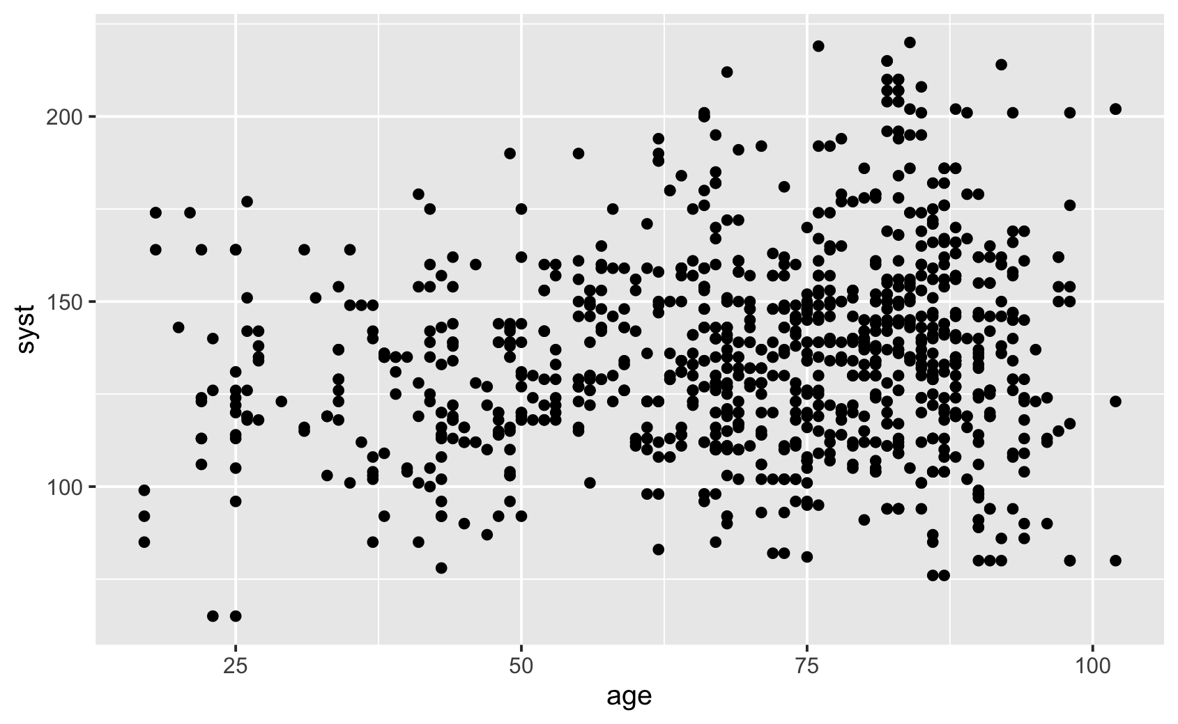
ggplot(news, aes(age, syst)) +
geom_point()Piirrä ikä ja systolinen verenpaine. Vaihda sitten y-akselille syke.
ggplot(news, aes(age, pulse)) +
  geom_point()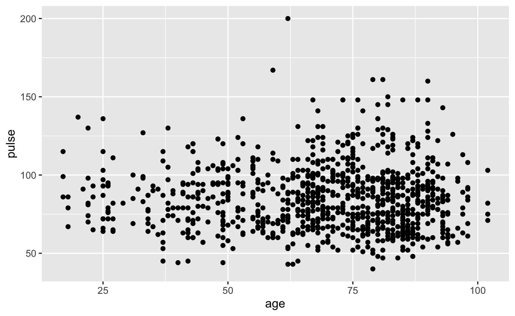
Väritä pisteet muuttujan mukaan tai anna kaikille sama väri. Säädä läpinäkyvyyttä ja vertaa tasoitettua käyrää suoraan.
ggplot(news, aes(age, syst, colour = sex)) +
  geom_point()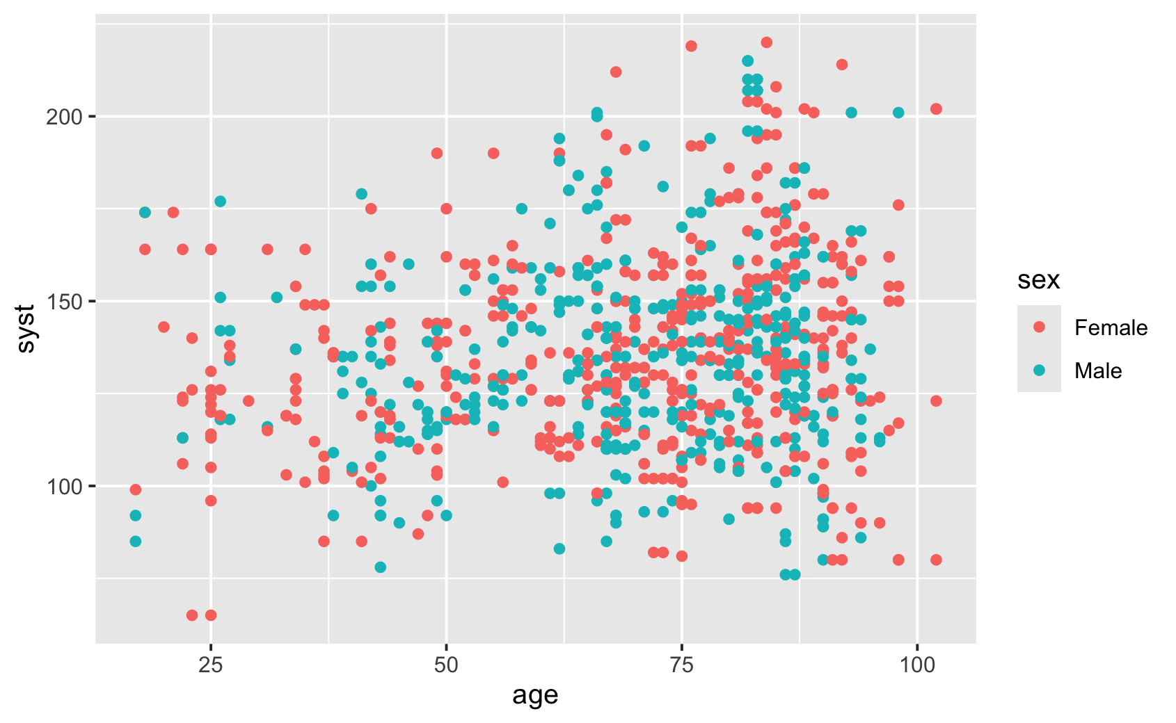
ggplot(news, aes(age, syst, colour = NEWS)) +
  geom_point()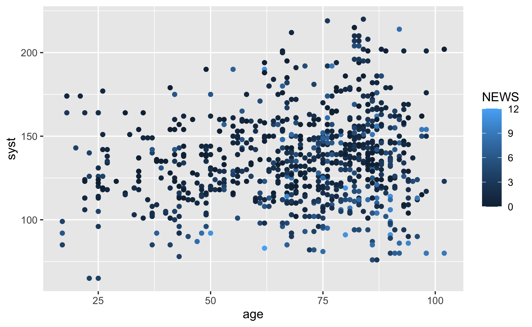
ggplot(news, aes(age, syst)) +
geom_point(colour = "steelblue")ggplot(
news,
aes(age, syst, colour = "steelblue")
) +
geom_point()ggplot(news, aes(age, syst)) +
geom_point(
colour = "steelblue",
alpha = 0.3
)ggplot(news, aes(age, syst)) +
geom_point() +
geom_smooth()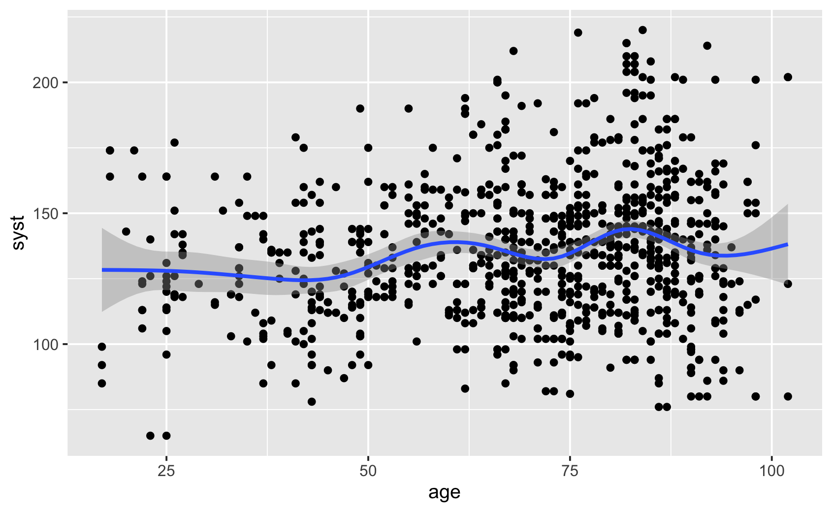
ggplot(news, aes(age, syst)) +
  geom_point() +
  geom_smooth(method = "lm")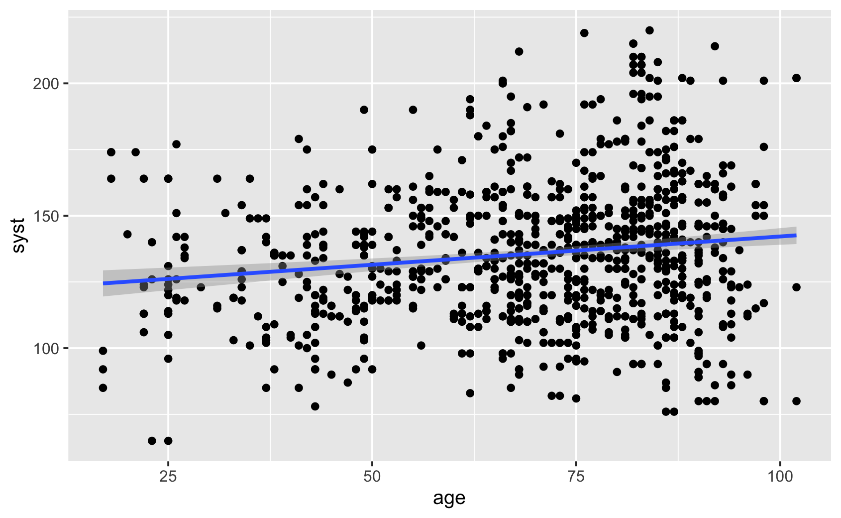
ggplot(news, aes(age, syst, colour = sex)) +
  geom_point() +
geom_smooth(method = "lm")ggplot(news, aes(age, syst)) +
geom_point(aes(colour = sex)) +
geom_smooth(method = "lm")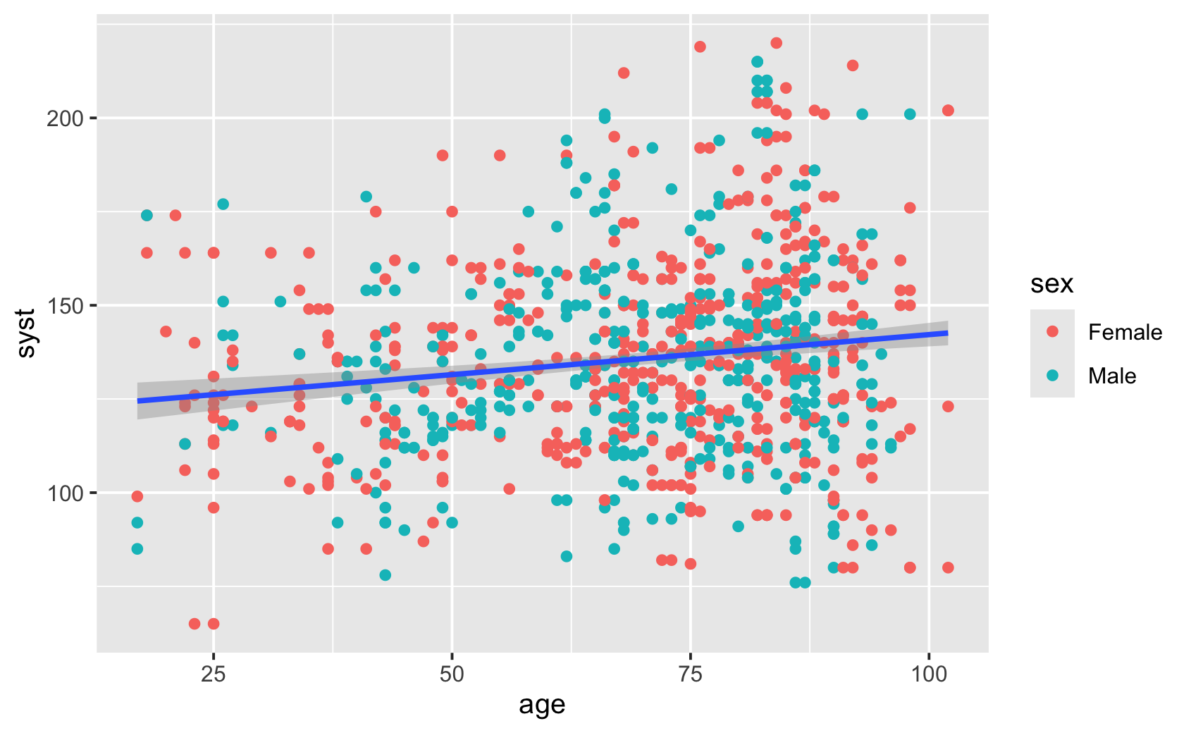
ggplot(news, aes(age, syst)) +
  geom_point() +
  geom_smooth(method = "lm") +
coord_cartesian(ylim = c(100, 150))ggplot(news, aes(age, syst)) +
geom_point() +
geom_smooth(method = "lm") +
ylim(100, 150)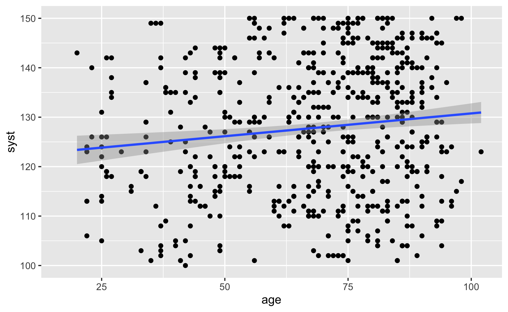
Piirrä ikä ja syke hajontakuvana. Väritä pisteet lisähapen (oxygen) mukaan.
ggplot(news, aes(age, pulse, colour = oxygen)) +
  geom_point()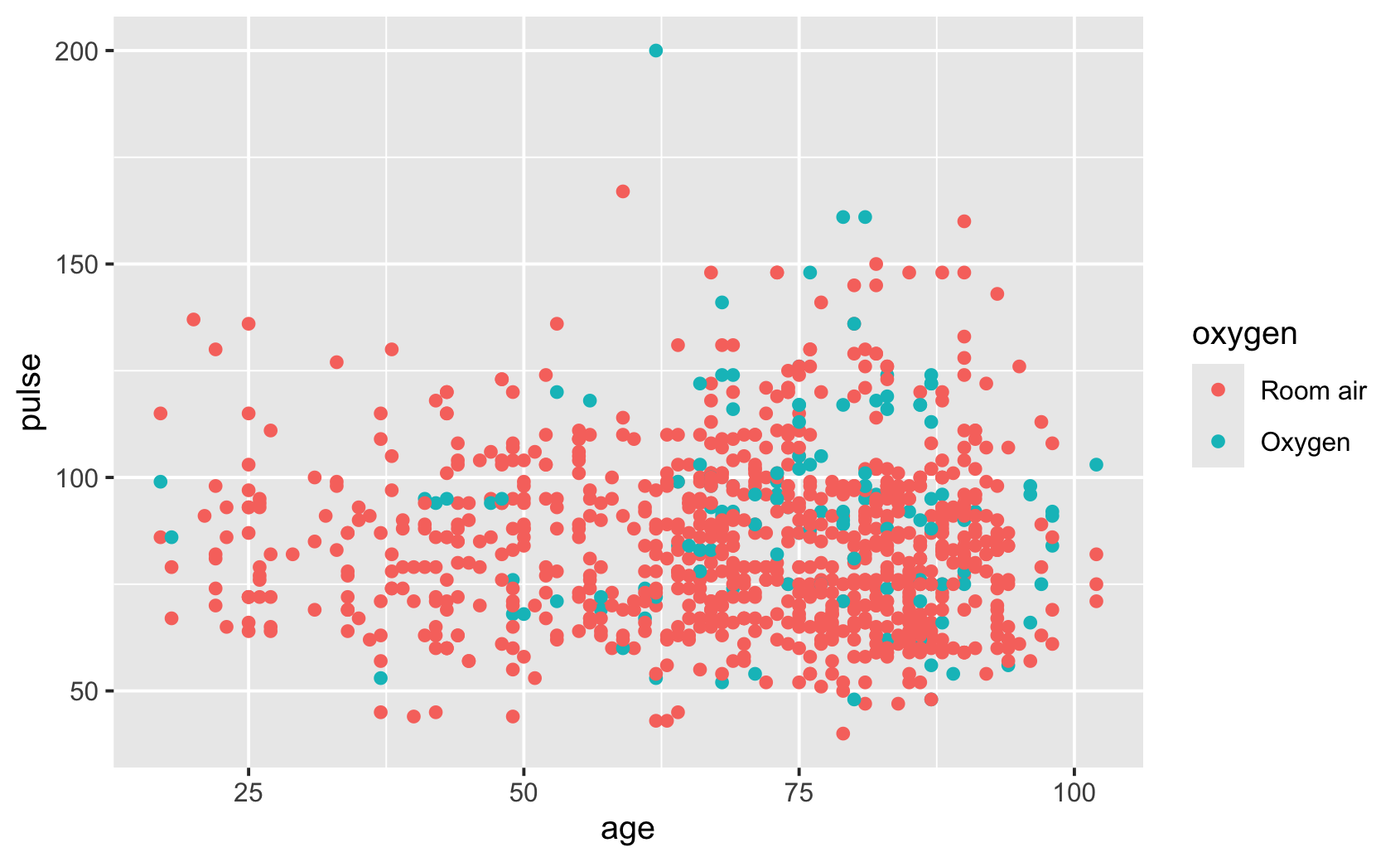
Säädä histogrammin pylvään leveyttä ja vertaile ryhmiä. Tiheyskuvaaja näyttää jakauman tasoitettuna.
ggplot(news, aes(age)) +
geom_histogram()ggplot(news, aes(age)) +
geom_histogram(binwidth = 5)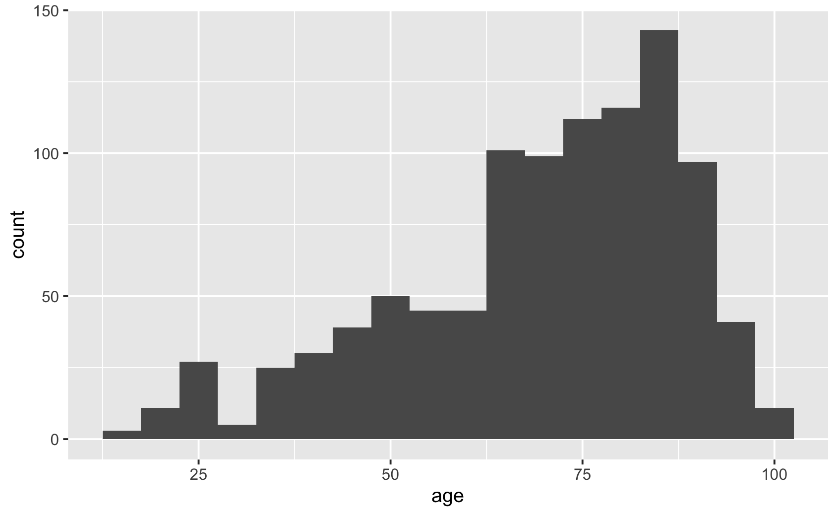
ggplot(news, aes(age)) +
geom_histogram(binwidth = 5, colour = "white")ggplot(news, aes(age, fill = sex)) +
geom_histogram(binwidth = 5, colour = "white")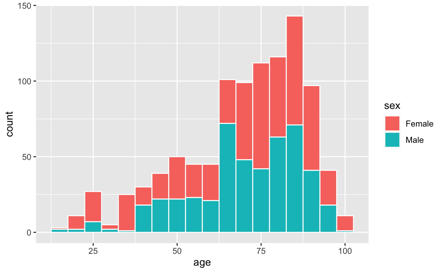
ggplot(news, aes(age, fill = sex)) +
geom_density()ggplot(news, aes(age, fill = sex)) +
geom_density(alpha = 0.4)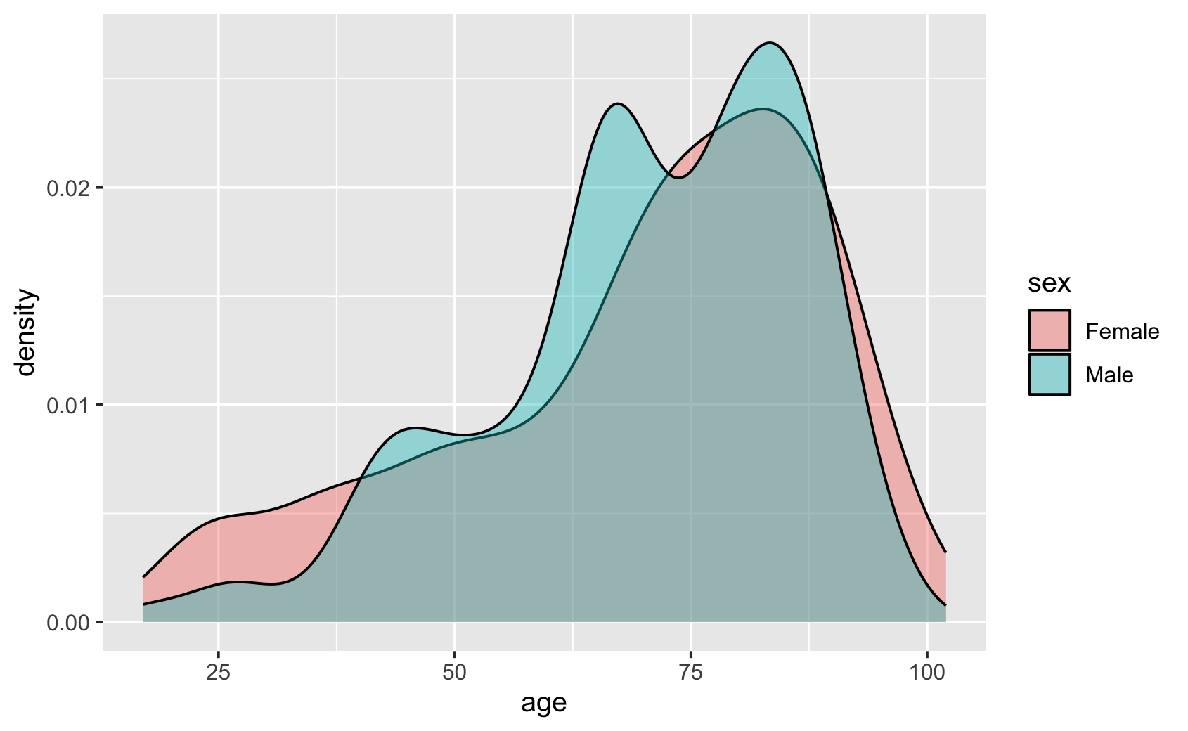
Piirrä diastolinen verenpaine (dias) histogrammina. Aseta pylväiden leveydeksi 5 mmHg.
ggplot(news, aes(dias)) +
  geom_histogram(binwidth = 5)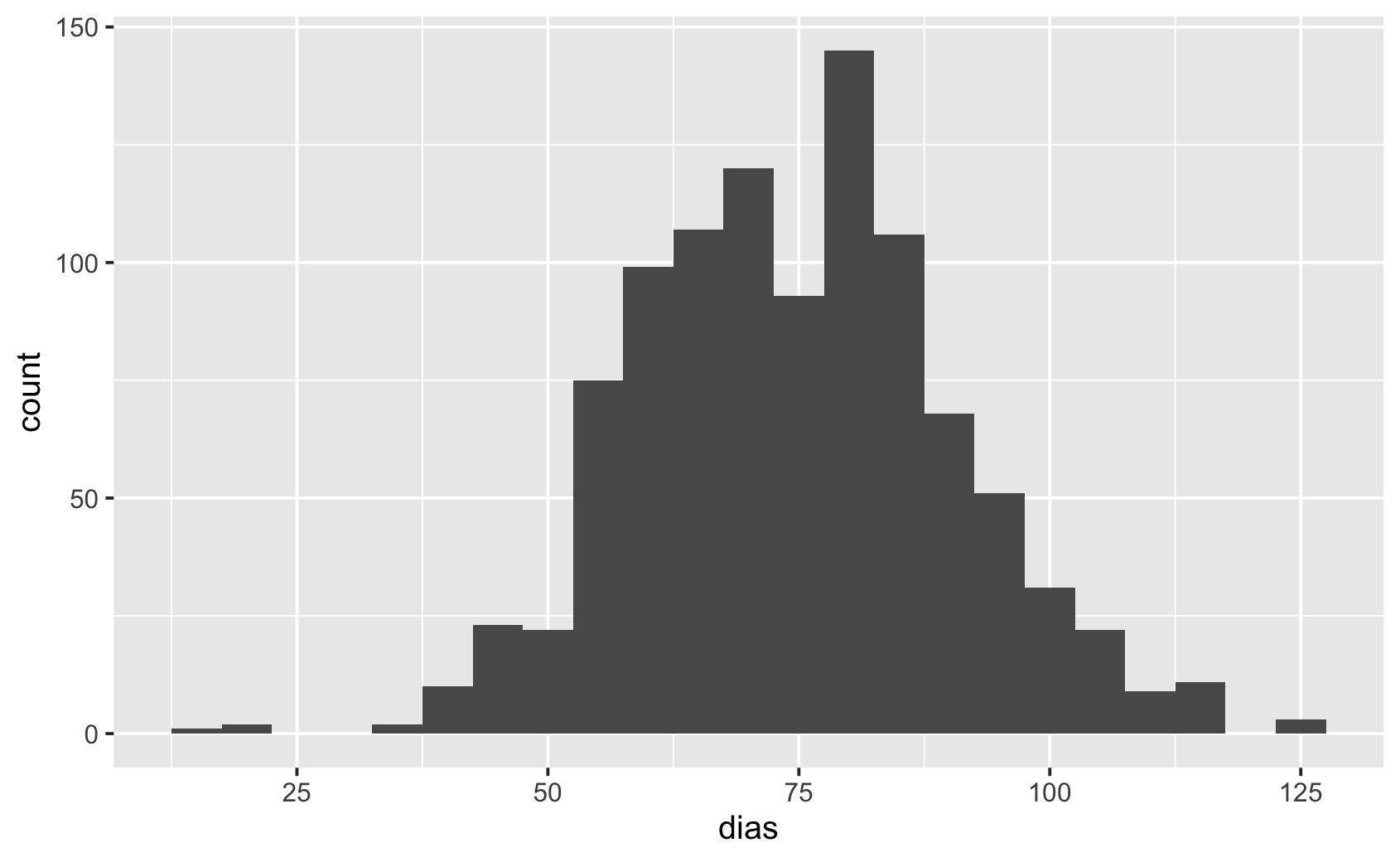
geom_bar() laskee ryhmien lukumäärät. Valinnalla position = "fill" kunkin pylvään kokonaiskorkeus on yksi.
ggplot(news, aes(oxygen)) +
  geom_bar()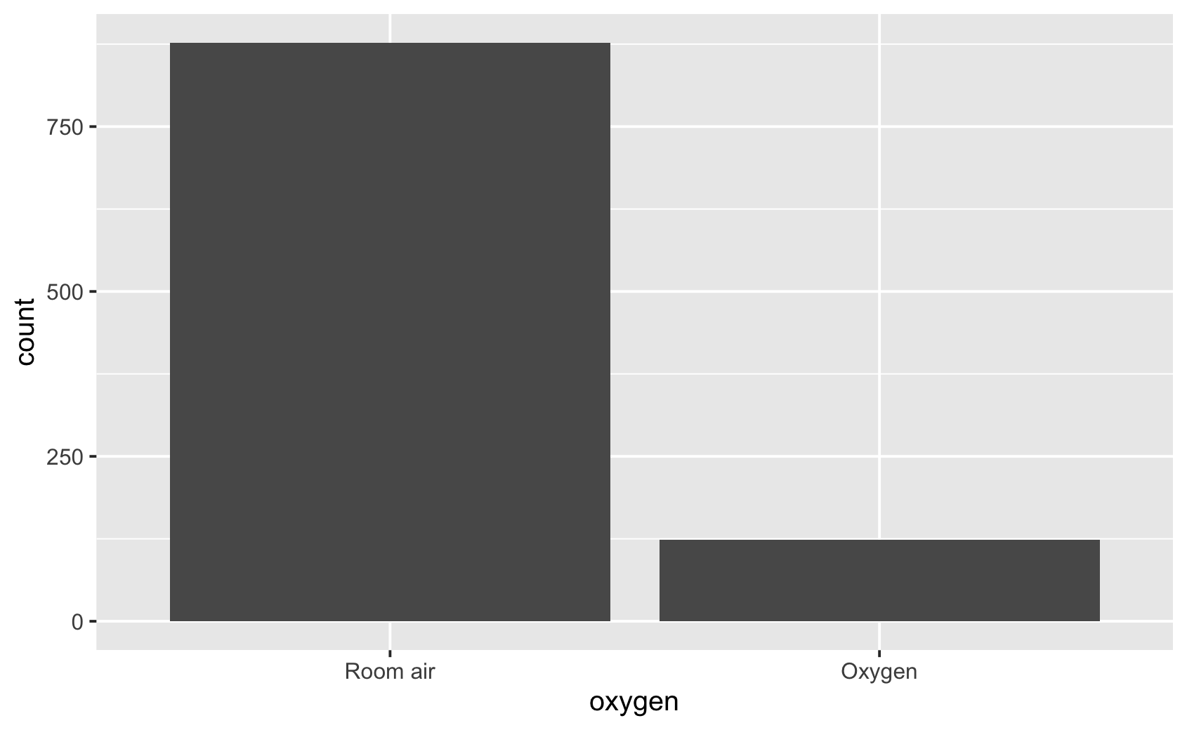
ggplot(news, aes(oxygen, colour = outcome)) +
geom_bar()ggplot(news, aes(oxygen, fill = outcome)) +
geom_bar()ggplot(news, aes(oxygen, fill = outcome)) +
geom_bar(position = "fill")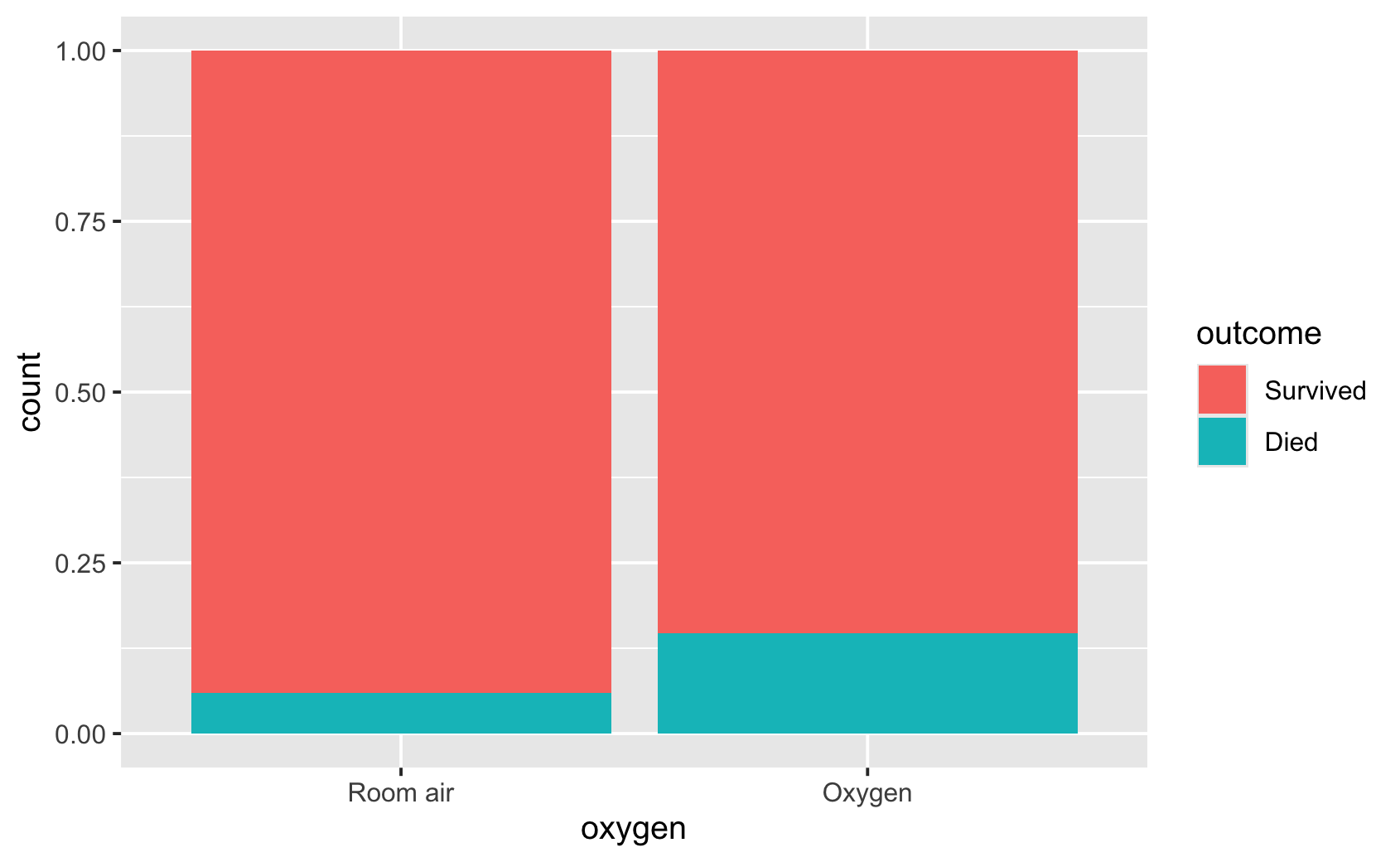
ggplot(news, aes(risk, fill = outcome)) +
  geom_bar(position = "fill")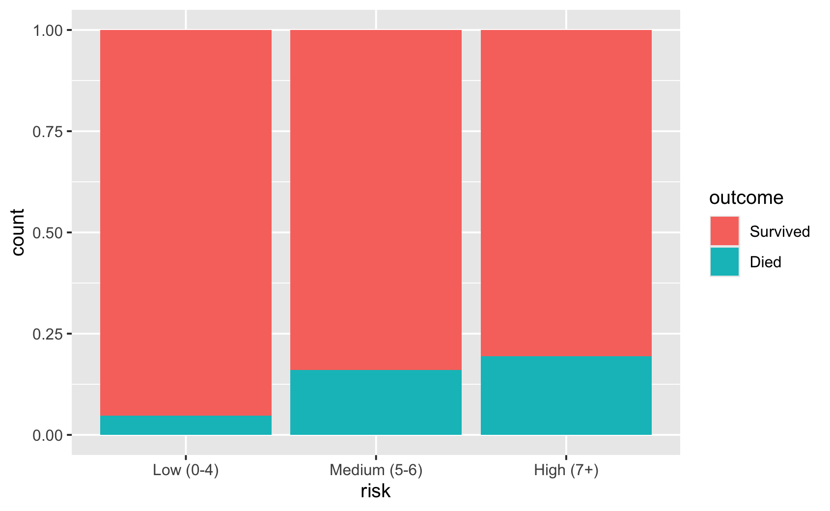
Rinnakkaiset pylväät ovat lisäesimerkki.
ggplot(news, aes(risk, fill = outcome)) +
  geom_bar(position = "dodge")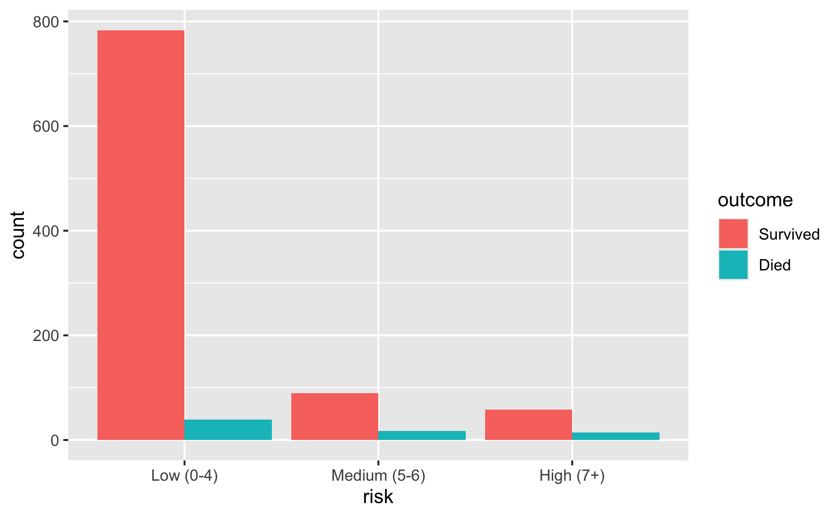
Vertaa sykkeen jakaumaa eri ryhmissä. Lisää yksittäiset havainnot ja tarkista ryhmäkoot.
ggplot(news, aes(outcome, pulse)) +
  geom_boxplot()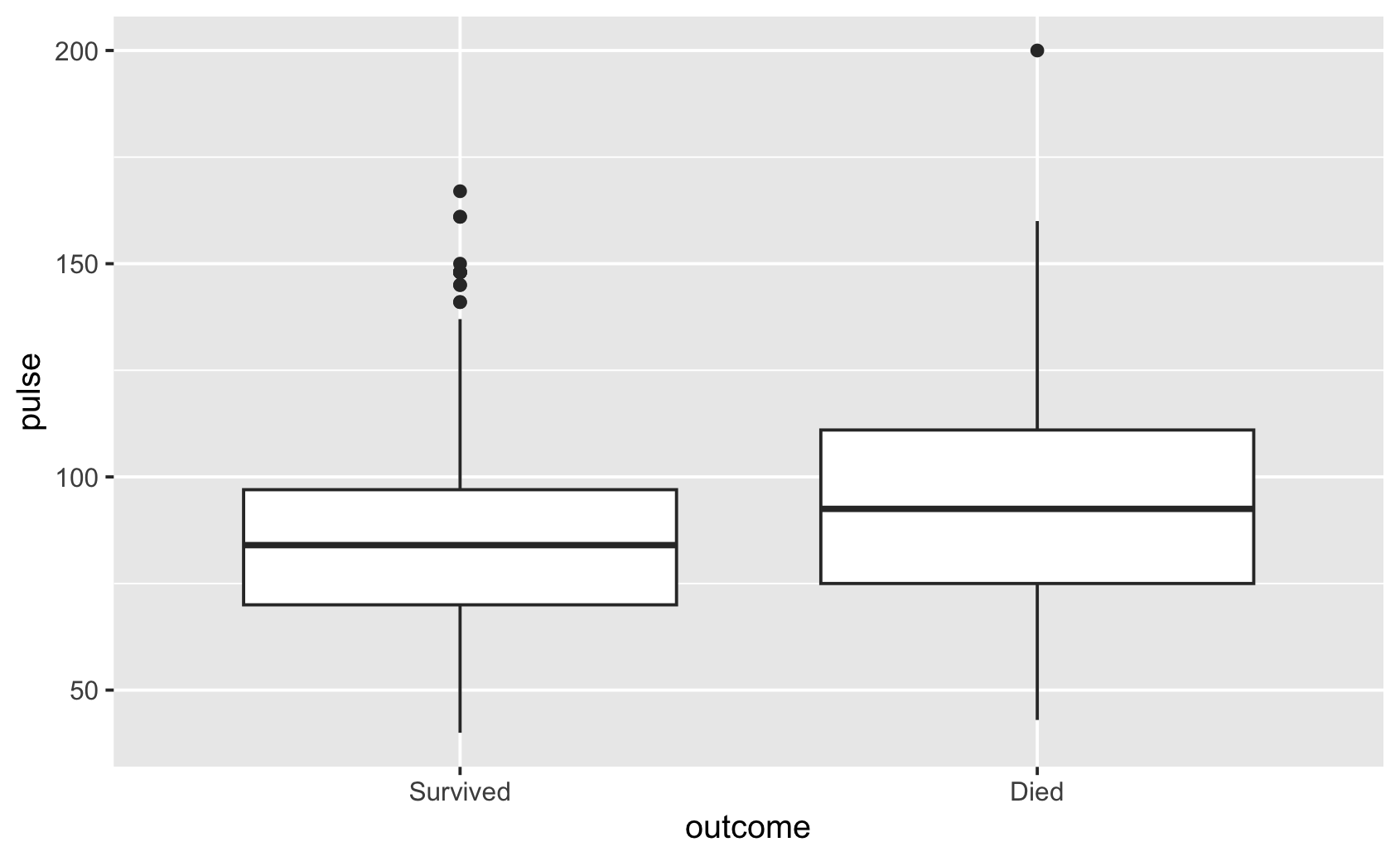
ggplot(news, aes(risk, pulse)) +
  geom_boxplot()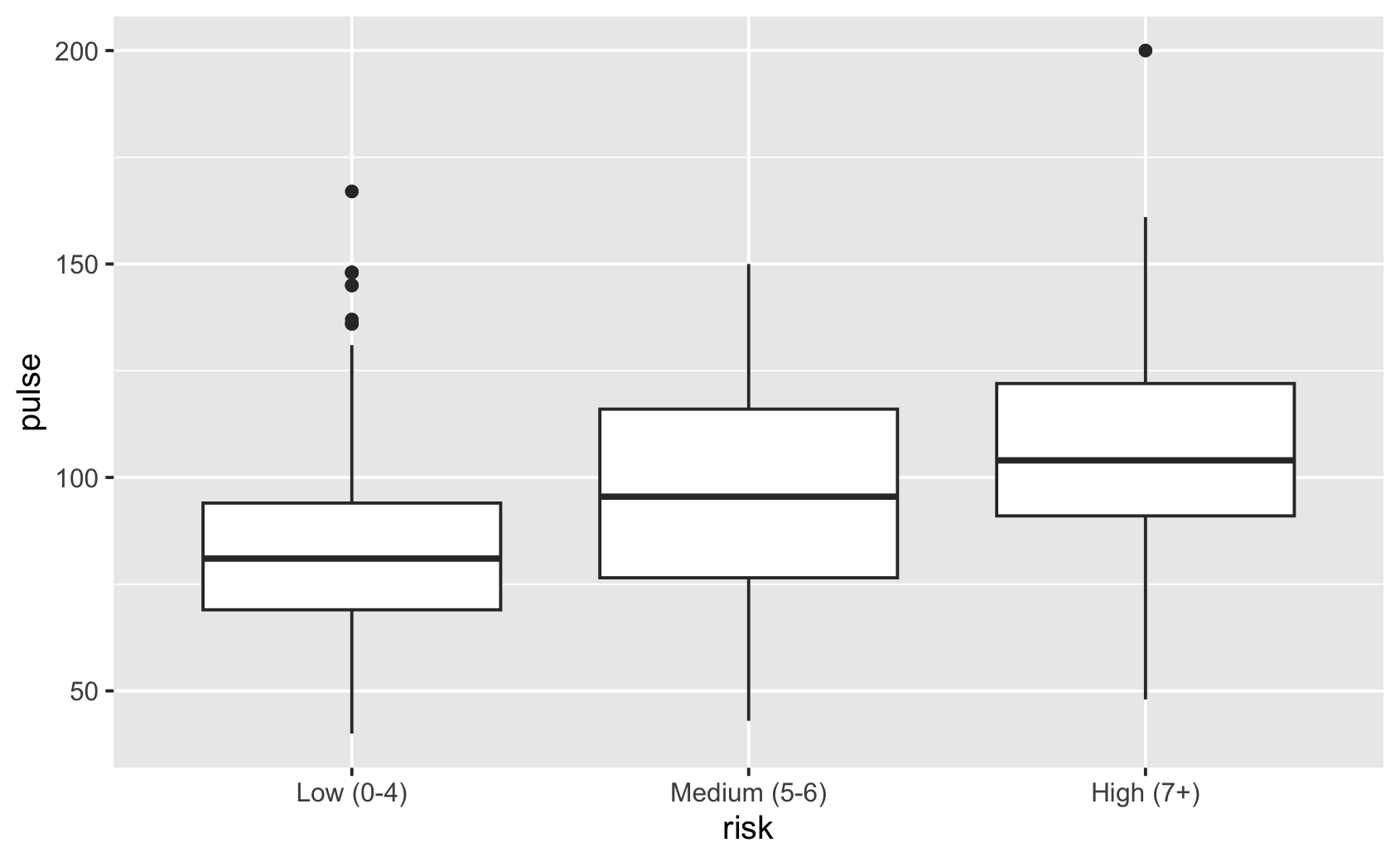
ggplot(news, aes(avpu, pulse)) +
geom_boxplot()ggplot(news, aes(avpu, pulse)) +
geom_boxplot() +
geom_jitter(width = 0.2, height = 0)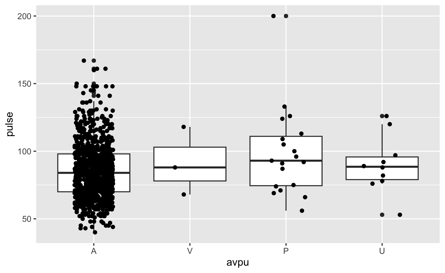
count(news, avpu)#> # A tibble: 4 × 2
#> avpu n
#> <fct> <int>
#> 1 A 968
#> 2 V 3
#> 3 P 19
#> 4 U 10Piirrä lämpötila (temp) NEWS-ryhmittäin (risk) laatikkokuviona.
ggplot(news, aes(risk, temp)) +
  geom_boxplot()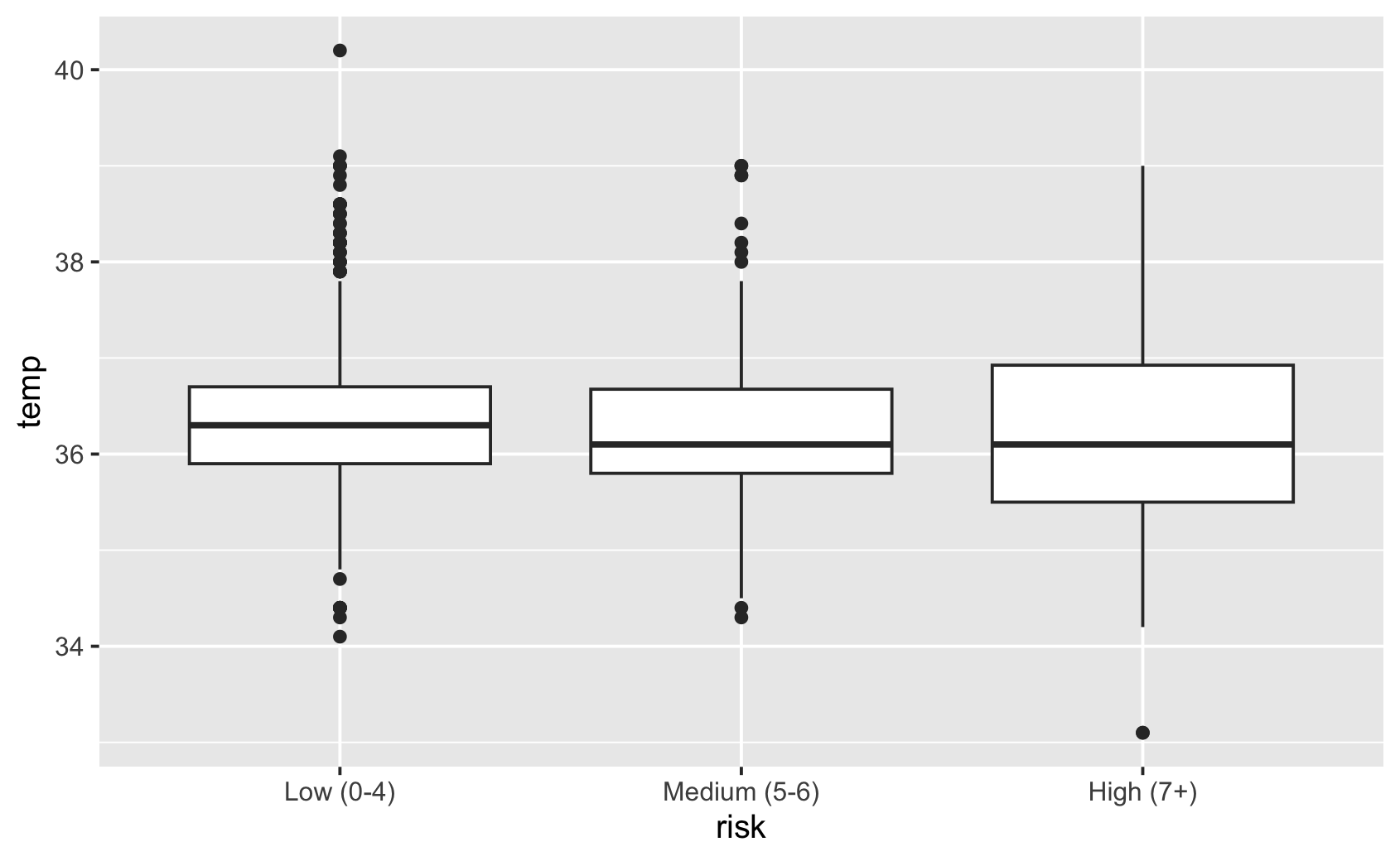
Piirrä kuolleiden osuus tajunnantason (avpu) mukaan. Tarkista, kuinka monesta havainnosta V-ryhmän osuus on laskettu.
ggplot(news, aes(avpu, fill = outcome)) +
  geom_bar(position = "fill")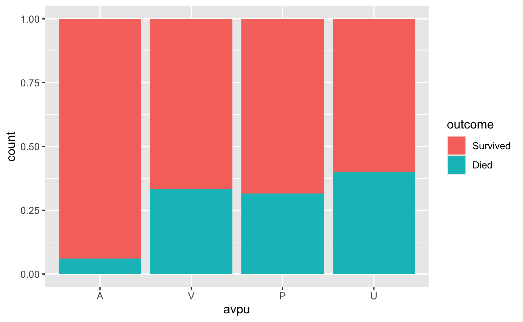
news |>
  filter(avpu == "V") |>
  count(outcome)
#> # A tibble: 2 × 2
#> outcome n
#> <fct> <int>
#> 1 Survived 2
#> 2 Died 1V-ryhmässä kuoli yksi kolmesta.
Kokeile pisteiden siirtämistä, muotoa ja kokoa. Piirrä kuolleiden osuutta kuvaava käyrä tai jaa havaintoja paneeleihin.
ggplot(news, aes(resp, sat)) +
geom_point()ggplot(news, aes(resp, sat)) +
geom_jitter()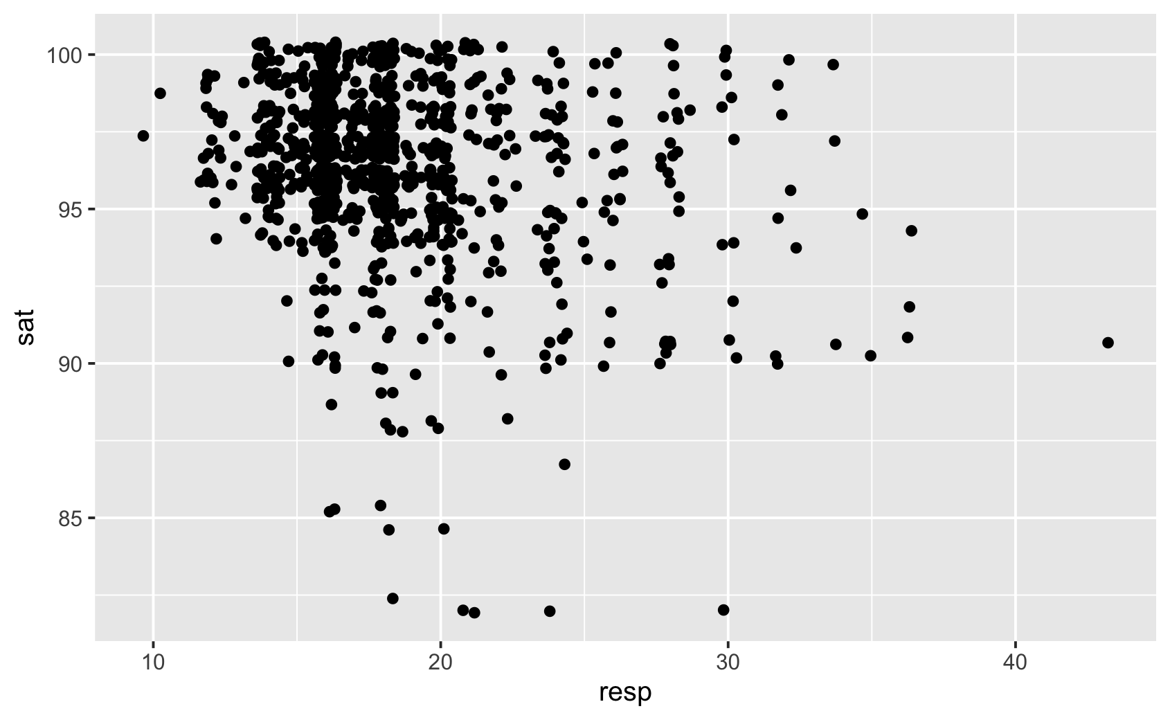
ggplot(news, aes(resp, sat, shape = oxygen)) +
geom_jitter()ggplot(news, aes(pulse, syst,
colour = outcome,
size = NEWS)) +
geom_point(alpha = 0.5)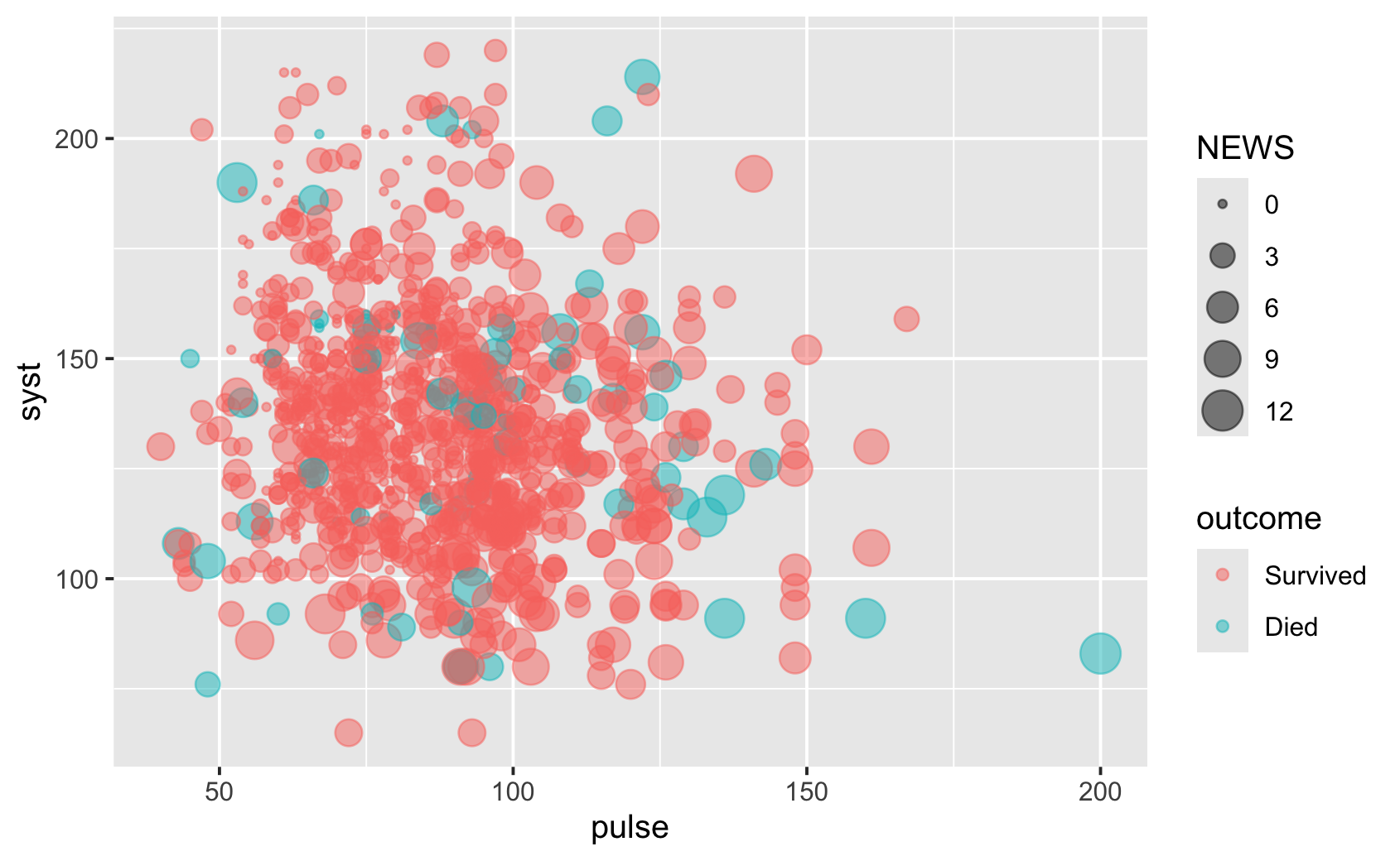
ggplot(news, aes(age, died)) +
  geom_point() +
  geom_smooth()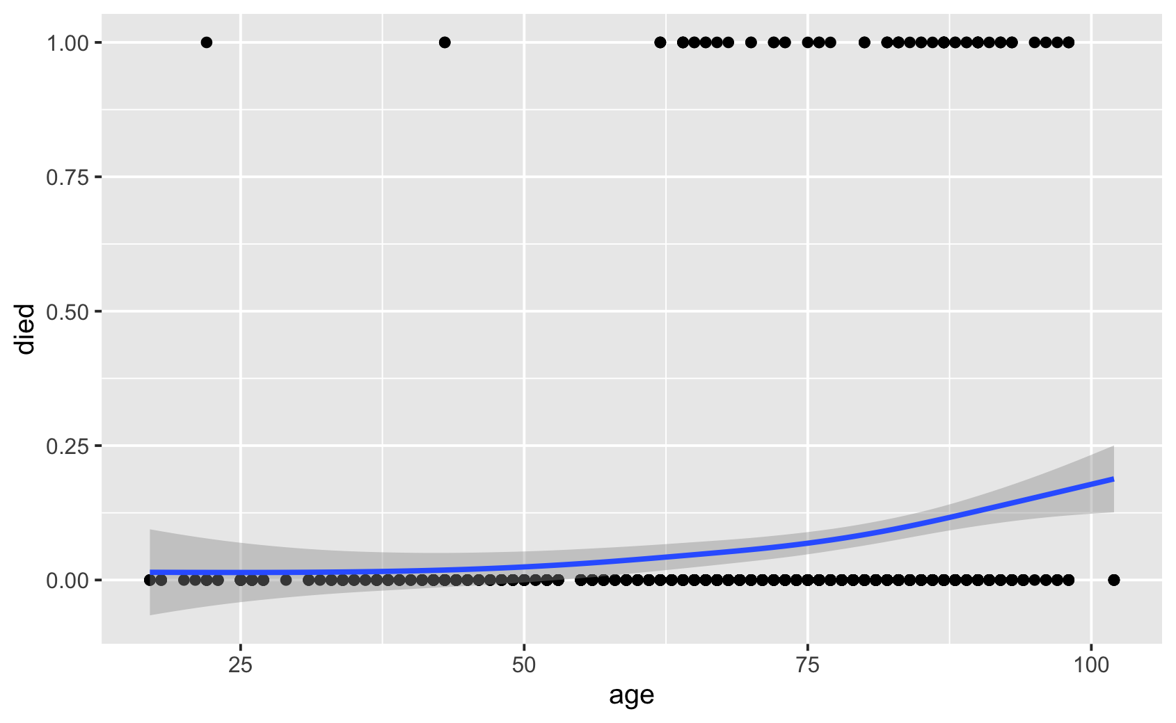
ggplot(news, aes(age, syst)) +
  geom_point() +
  facet_wrap(vars(risk))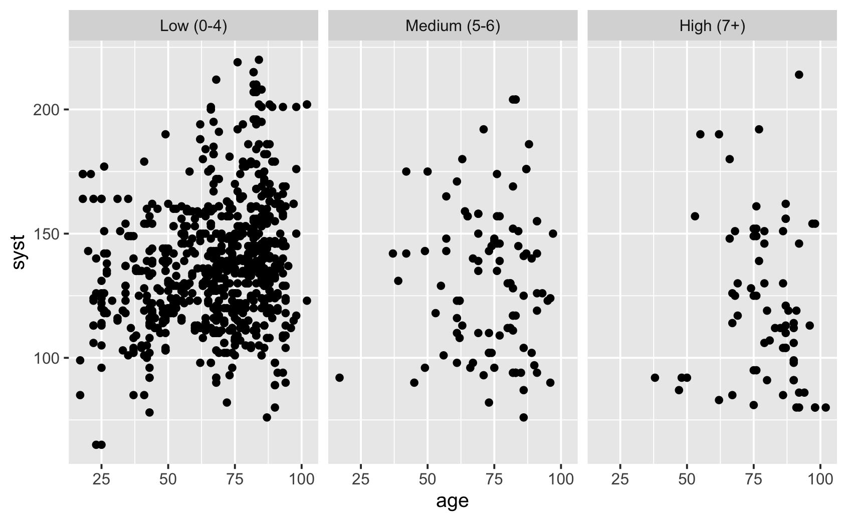
Lisää akselien nimet, otsikko ja lähde. Vaihda teema ja aja tallennuskomento omassa Positron-istunnossasi heti kuvaajan piirtämisen jälkeen.
ggplot(news, aes(age, syst, colour = sex)) +
  geom_point() +
geom_smooth(method = "lm")ggplot(news, aes(age, syst, colour = sex)) +
geom_point() +
geom_smooth(method = "lm") +
labs(
x = "Age (years)",
y = "Systolic blood pressure (mmHg)"
)ggplot(news, aes(age, syst, colour = sex)) +
geom_point() +
geom_smooth(method = "lm") +
labs(
x = "Age (years)",
y = "Systolic blood pressure (mmHg)",
colour = "Sex",
title = "Age and systolic blood pressure",
subtitle = "Synthetic hospital data",
caption = "Source: NHSRdatasets"
)ggplot(news, aes(age, syst, colour = sex)) +
geom_point() +
geom_smooth(method = "lm") +
labs(
x = "Age (years)",
y = "Systolic blood pressure (mmHg)",
colour = "Sex",
title = "Age and systolic blood pressure",
subtitle = "Synthetic hospital data",
caption = "Source: NHSRdatasets"
) +
theme_minimal()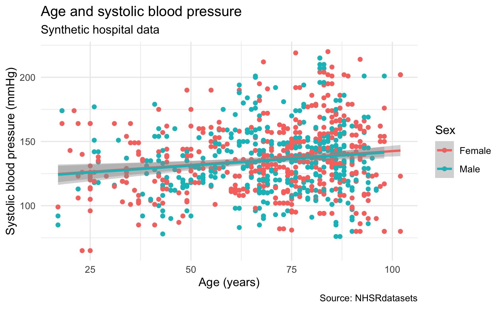
ggsave(
  "age_syst.png",
  width = 7, height = 5, dpi = 300
)Piirrä ikäjakauma eloonjääneille ja kuolleille tiheyskuvaajana. Lisää otsikko ja akselien nimet, vaihda teema ja tallenna kuva.
ggplot(news, aes(age, fill = outcome)) +
  geom_density(alpha = 0.4) +
  labs(
    x = "Age (years)",
    y = "Density",
    fill = "Outcome",
    title = "Age distribution by outcome",
    subtitle = "Synthetic teaching data"
  ) +
  theme_minimal()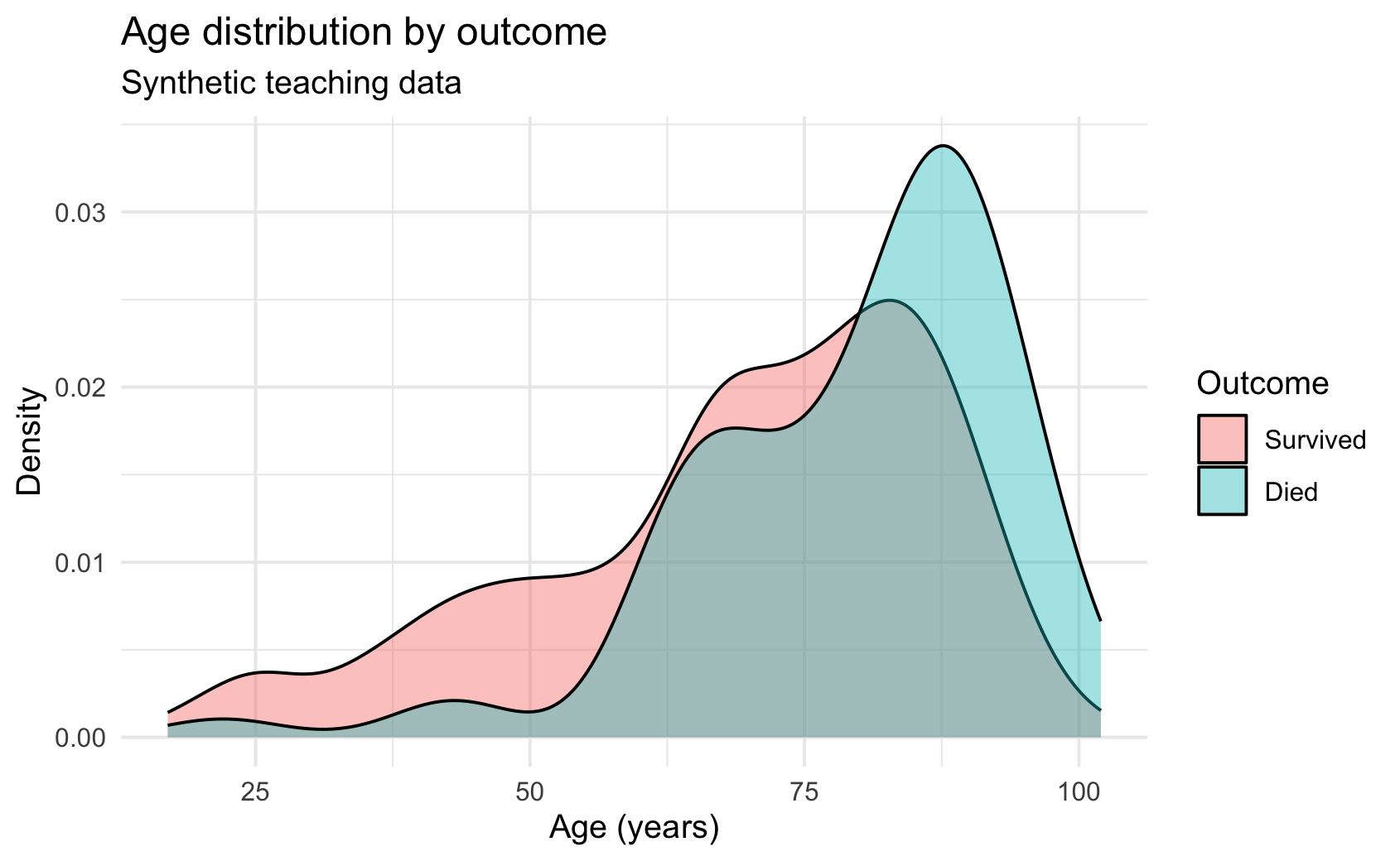
ggsave(
  "age_distribution.png",
  width = 7, height = 5, dpi = 300
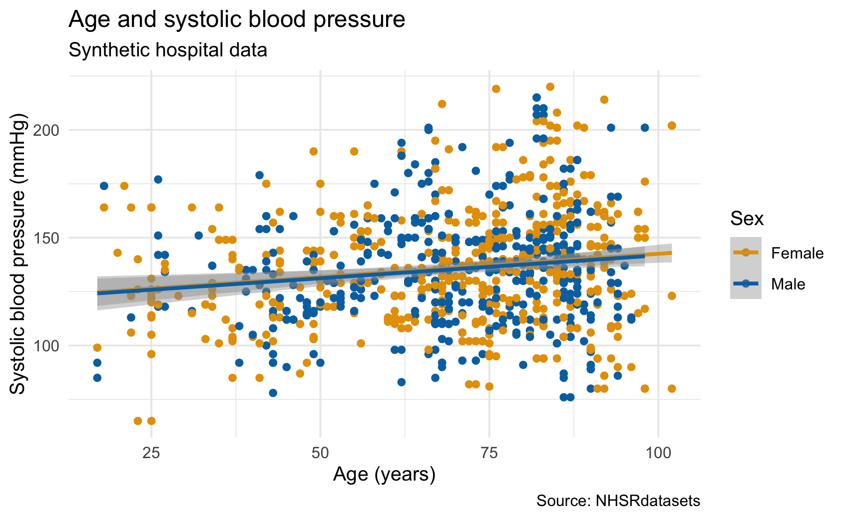
)ggplot(news, aes(age, syst, colour = sex)) +
geom_point() +
geom_smooth(method = "lm") +
labs(
x = "Age (years)",
y = "Systolic blood pressure (mmHg)",
colour = "Sex",
title = "Age and systolic blood pressure",
subtitle = "Synthetic hospital data",
caption = "Source: NHSRdatasets"
) +
theme_minimal() +
scale_colour_manual(
values = c(
Female = "#E69F00",
Male = "#0072B2"
)
)
ggplot(news, aes(risk, fill = outcome)) +
  geom_bar(position = "fill") +
  labs(y = "Proportion") +
  scale_fill_brewer(palette = "Set2")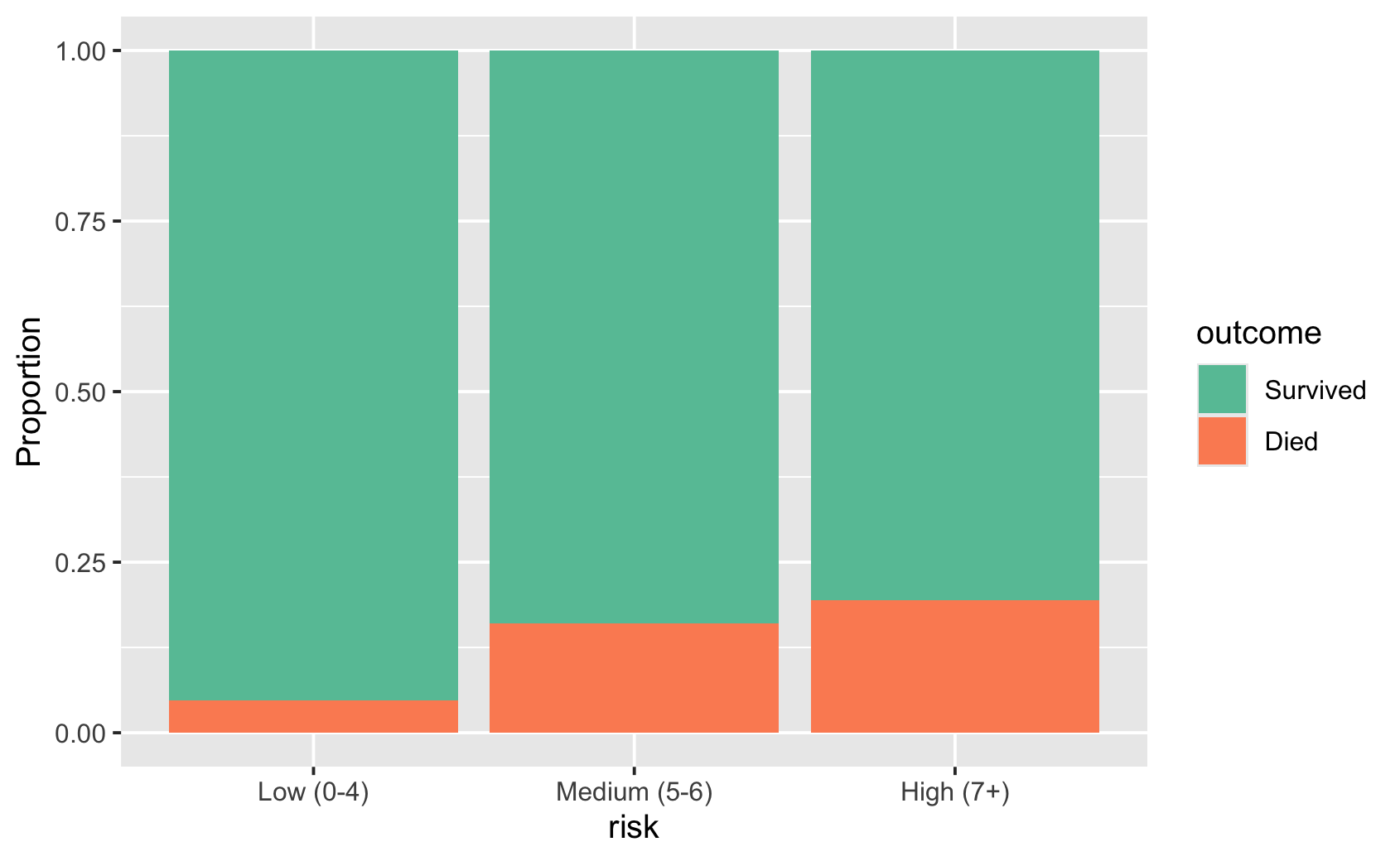
ggplot(news, aes(age, syst, colour = NEWS)) +
  geom_point() +
  scale_colour_viridis_c()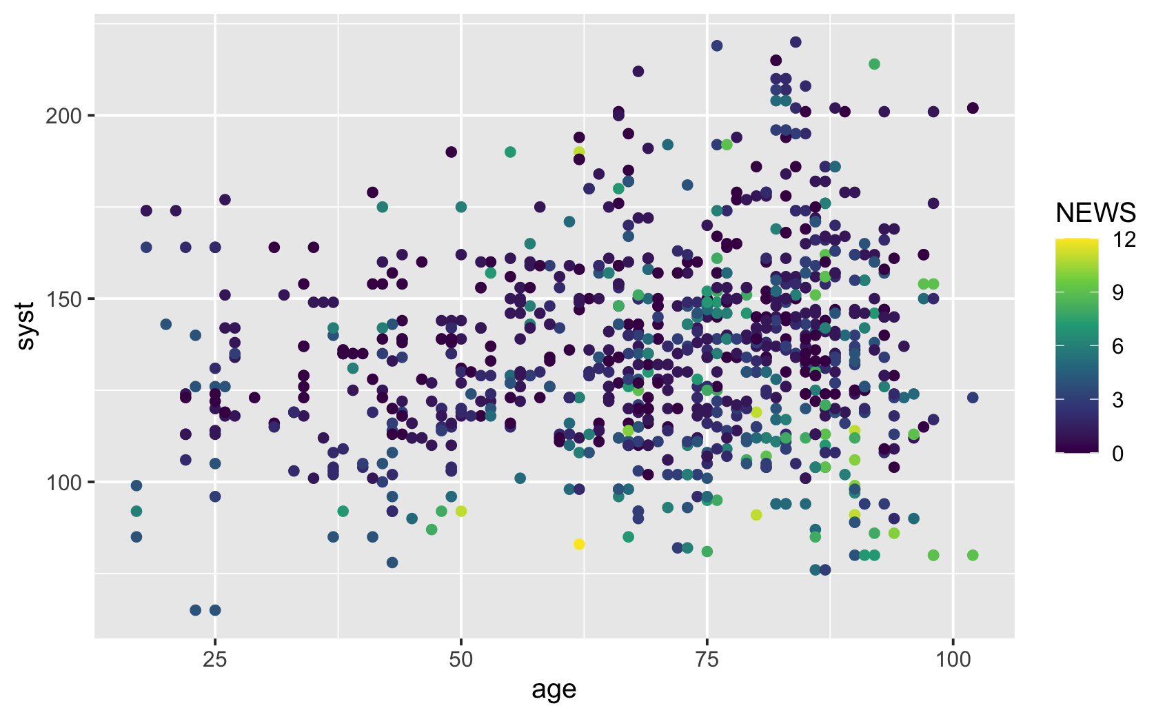
Katso kuvaajaa ja mieti, millä koodilla tekisit sen. Avaa mallikoodi yrityksen jälkeen.
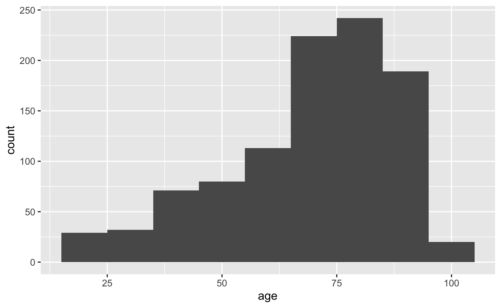
ggplot(news, aes(age)) +
  geom_histogram(binwidth = 10)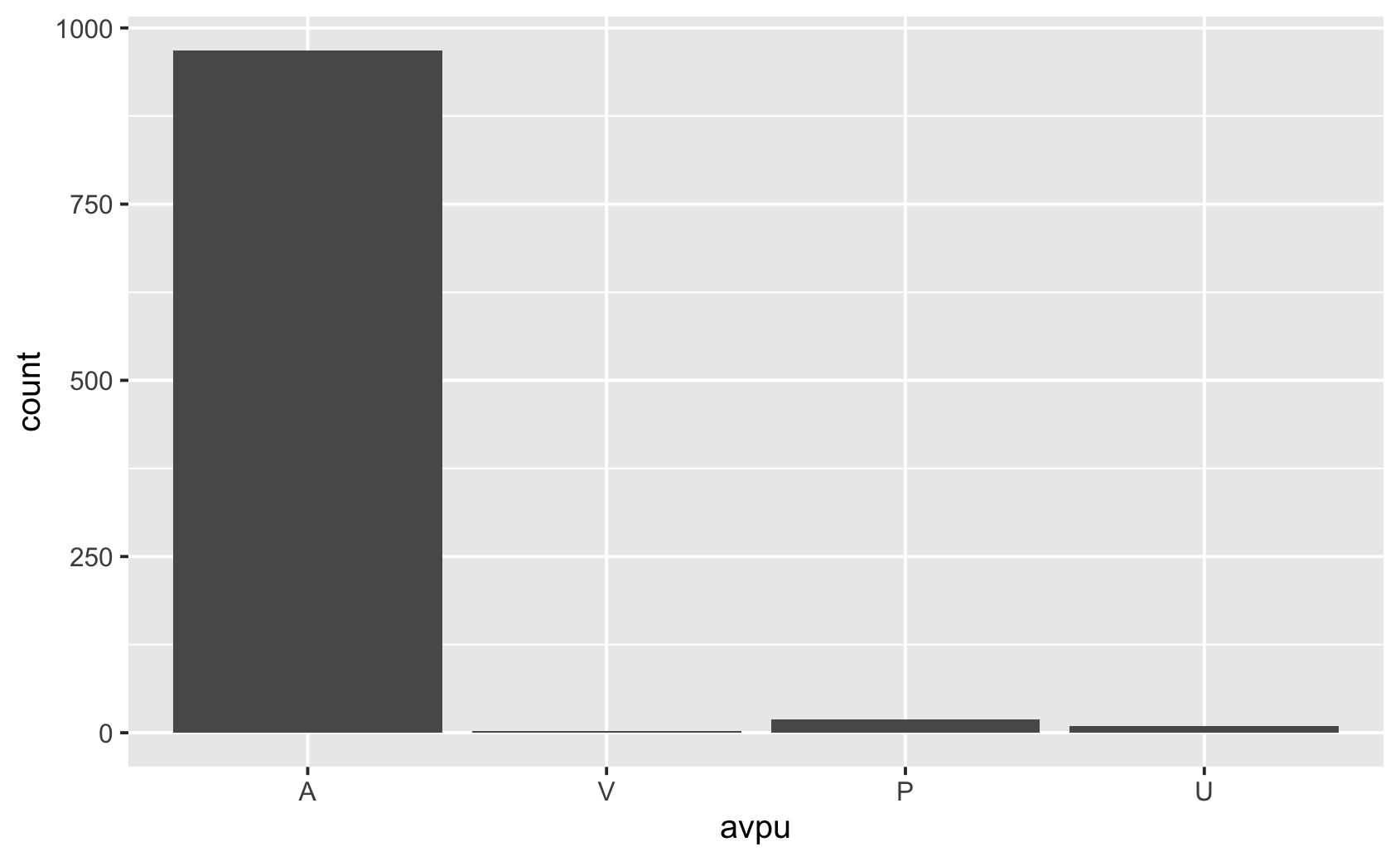
ggplot(news, aes(avpu)) +
  geom_bar()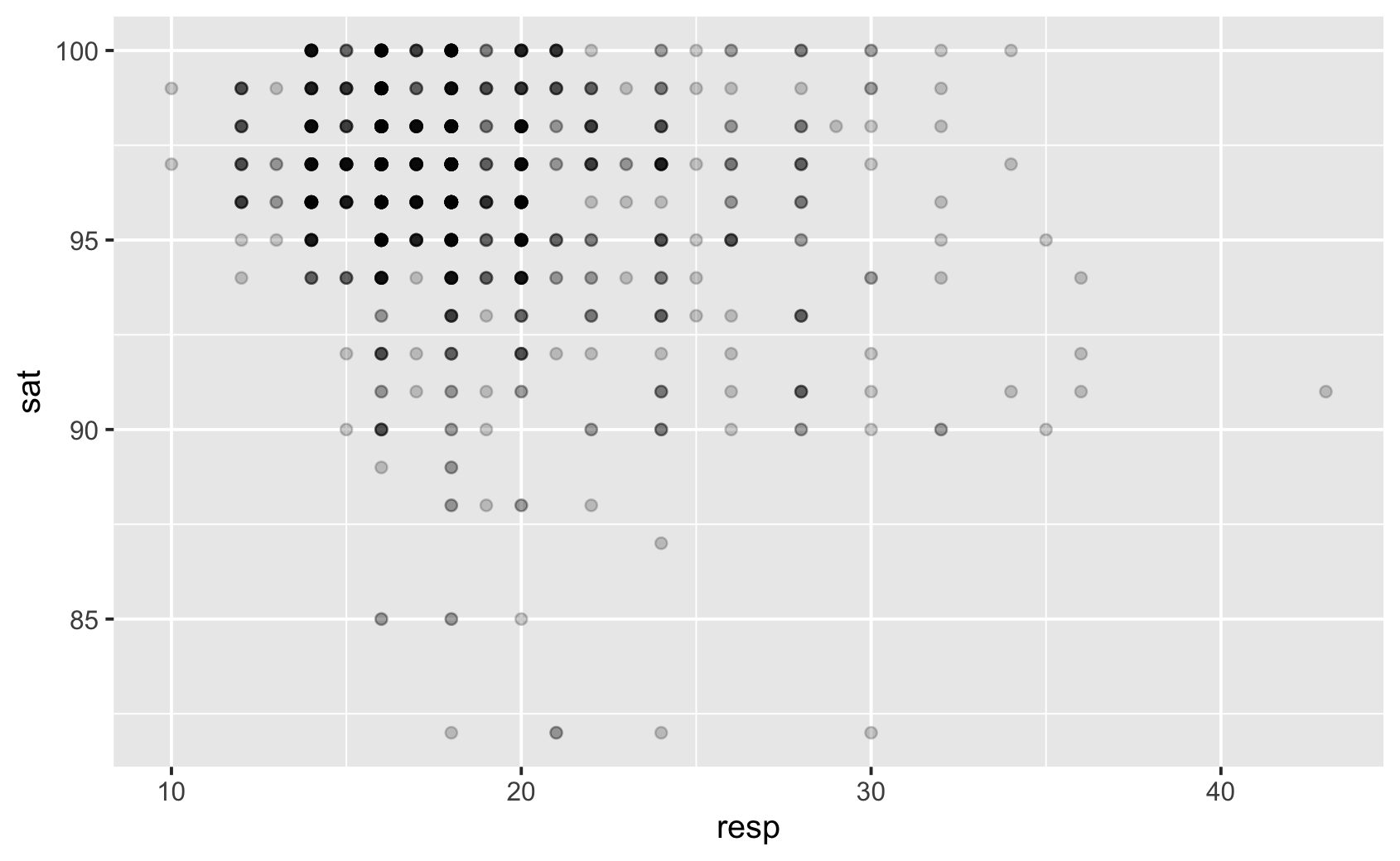
ggplot(news, aes(resp, sat)) +
  geom_point(alpha = 0.2)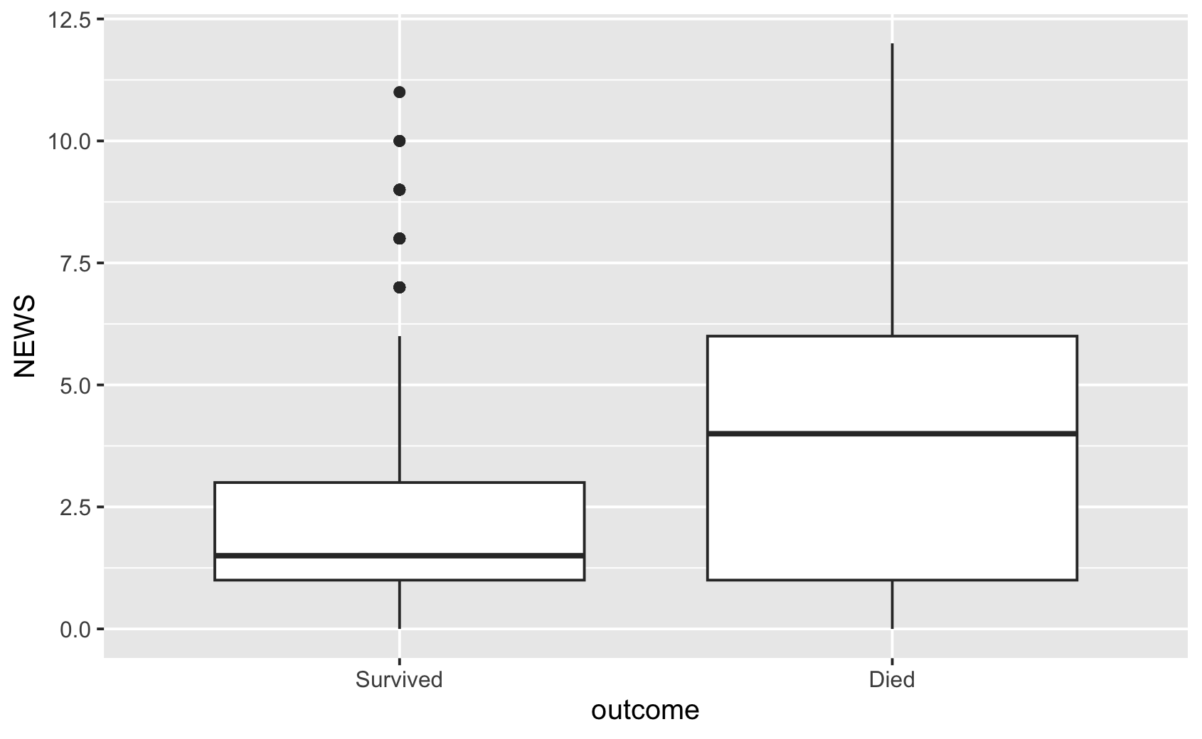
ggplot(news, aes(outcome, NEWS)) +
  geom_boxplot()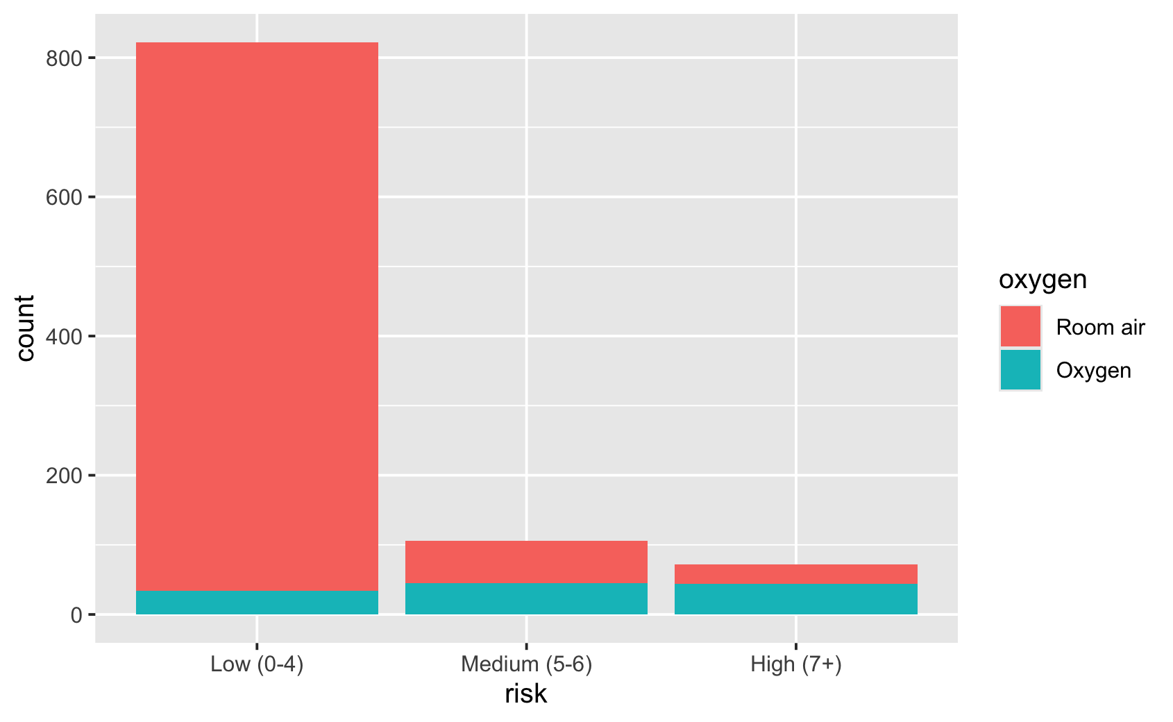
ggplot(news, aes(risk, fill = oxygen)) +
  geom_bar()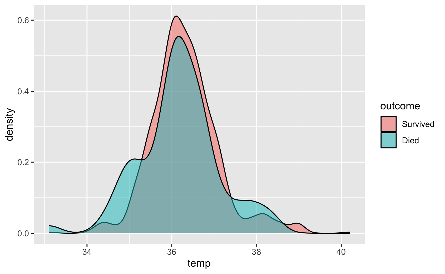
ggplot(news, aes(temp, fill = outcome)) +
  geom_density(alpha = 0.5)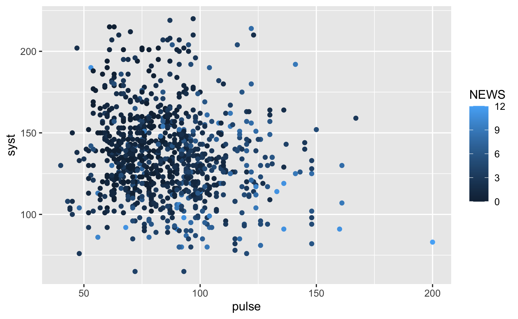
ggplot(news, aes(pulse, syst, colour = NEWS)) +
  geom_point()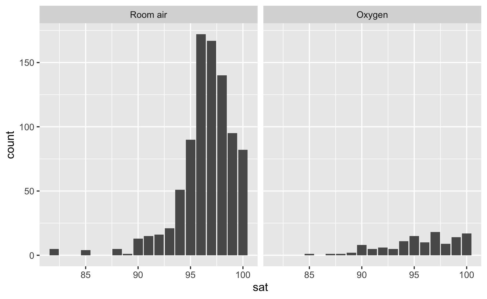
ggplot(news, aes(sat)) +
  geom_bar() +
  facet_wrap(vars(oxygen))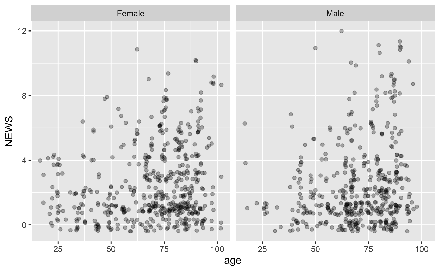
ggplot(news, aes(age, NEWS)) +
  geom_jitter(alpha = 0.3) +
  facet_wrap(vars(sex))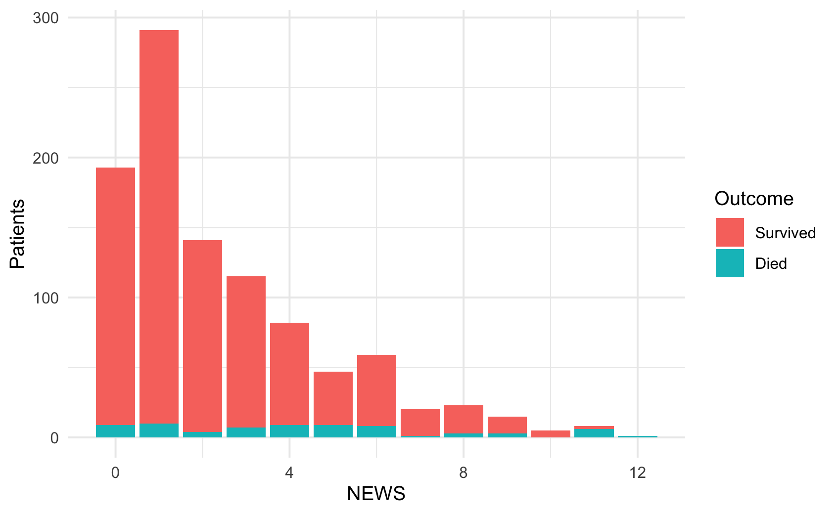
ggplot(news, aes(NEWS, fill = outcome)) +
  geom_bar() +
  labs(
    x = "NEWS",
    y = "Patients",
    fill = "Outcome"
  ) +
  theme_minimal()